Converting a Kaggle notebook to a Kedro Pipeline
This tutorial is aimed at Data Scientists who want to convert Jupyter Notebook to a Kedro pipeline. Notebooks are a great way to experiment and explore data, figure out what machine learning model works well and illustrate outcomes. But it is very hard to maintain notebooks, they don’t play nice with repositories, testing can’t be automated and you can’t reuse code from them or integrate them into a bigger workflow. So Kedro takes all these good things we have learned from software engineering and applies them to data science projects. But how to get started?
We will be using a Kaggle notebook project as example and convert it to a Kedro pipeline. Along the way I will aim to illustrate the steps you should consider and why they are important.
Prerequisites
If you want to follow along you need to install Jupyter Notebook or Jupyter Lab as well as Kedro. All the examples use VS Code. An ideal starting point is the end of my tutorial on Setting up a Virtual Environment and VS Code for Kedro . It guides you through from start to having a blank, working Kedro project. The examples are from a Windows environment, so there may be subtle differences for Mac users. I have also prepared a branch with the output from this tutorial which you can clone using:
git clone --branch empty_kedro_project https://github.com/picklejuicedev/kedro-tutorial.git
Remember to create a virtual environment and install all the dependencies using:
pip install -r src/requirements.txt
The notebook
If you like, please download this notebook and the data. Feel free to explore, it is a pretty basic ML project, taken from the Kaggle starter competition “Spaceship Titanic”.
Initially it will install the missing pandas and scikit-learn packages. After loading the data, we do some pre-processing, figuring out if a passenger was travelling alone or in a group. Next, we take care of NaN values. Clearly there is more pre-processing we could do, but let’s keep it simple.
We then use a LabelEncoder to convert some label columns in to integer values and delete uneccessary columns.
Next we split the data into training and test sets and train a RandomForrestClassifier.
Last but not least we print a report with how it is performing.
If you run this notebook it will create some results like this:
---------- RandomForest ----------
Accuracy = 77.84 %
Precision = 78.11 %
Recall = 75.65 %
F1-Score = 76.86 %
Analysing the structure
Before creating a Kedro project, let’s establish what the different parts of the pipeline would be. A good starting point is:
- Pre-processing
- Encoding
- Make a model
- Reporting
I have already annotated the notebook with some of those functions, but we want to create processing blocks or nodes that do each task. This way we can
- test and debug each task
- they have a clearly defined input and output (or interface)
- which means we can then easily swap them out with alternative processing blocks
- connect building blocks to create a pipeline
- that can run locally as well as remotely
- can be triggered or scheduled
- can be fed different inputs if we need to update the model
So these and more are the benefits when moving to Kedro.
Project setup
Let’s start with a blank Kedro project, if you need any help, check out the Kedro documentation or my article on Setting up a Virtual Environment and VS Code for Kedro .
As a starting point we want to copy 2 files into the project folder:
- first, copy
train.csvtodata/01_raw/ - then, copy the notebook into the folder
notebooks/
We need to install the pandas and scikit-learn packages that will be used by the project:
pip install pandas scikit-learn
Next, open up VS code if not already running. Be sure to have the virtual environment with all dependencies as interpreter.
Registering the data file
Before we register the csv file in the project catalog, let’s look at the reasoning behind having a YAML file for this. After all, we could just reference it directly as in the notebook, right? But let’s imagine moving this project to a cloud server, then the file reference will change as the file may be located somewhere else. Or the name changes. Or you are given a parquet file instead of a csv file. In all these cases you would simply edit the catalog.yml file and don’t need to touch any code. This makes it easier to adapt and less likely to break. For the same reason user configurable parameters are saved in the parameters.yml file. Or logging details in logging.yml. I think you get the idea, it simply makes good sense to move anything that frequently changes into a settings file so it can be modified without updating the code.
Open conf/base/catalog.yml and add:
#catalog.yml

train:
  type: pandas.CSVDataSet
  filepath: data/01_raw/train.csv
Let’s load this now in our notebook. As we are in VS Code, we can open a new integrated terminal (right click in explorer), then use the kedro jupyter lab command to start the notebook editor. Once inside, change the loading of the data from using pandas to catalog.load:
Please note that if the catalog doesn’t load then you need to change the kernel for the notebook to the one labelled “Kedro(kedro_project)”. Kedro “injects” the catalog and other variables into the kernel so they are accessible by the notebook. Whilst VS Code can run Jupyter Notebooks inside the editor there can be problems with injecting the Kedro variables. So we’ll stick to running notebooks the classic way.
To shut down the Jupyter lab server, press crtl + C twice in the terminal window. For now, just leave it running as we will move some code around.
Converting code blocks into functions
We can now create a new pipeline in Kedro and start moving the code from the Jupyter Cells into dedicated functions which will become nodes. Let’s go through the steps first and then discuss why this is useful after.
A pipeline is a data processing flow, it takes input datasets like our csv file and passes it through various nodes, each doing one step of the processing, until you have an output at the end. In our case it will simply print the results to the log.
Let’s create a pipeline called data_proc in the command line:
kedro pipeline create data_proc
This will create empty files for us to populate. Open src/kedro_project/pipelines/data_proc/nodes.py.
We will take the two pre-processing cells from the notebook and copy them over, then make functions out of them:
# pipelines/data_proc/nodes.py

import pandas as pd

def compute_group_size(df_train: pd.DataFrame) -> pd.DataFrame:
    """
    Args:
        df_train (pandas.DataFrame): Dataframe with training data.

    Returns:
        pandas.DataFrame: Dataframe with training data and group size.
    """
    split_df = df_train["PassengerId"].str.split(pat="_", expand=True)
    alone = split_df[0].value_counts()
    split_df = split_df.merge(alone.rename("groupSize"), left_on=0, right_index=True)
    df_train["groupSize"] = split_df["groupSize"]
    return df_train


def resolve_na(df_train: pd.DataFrame) -> pd.DataFrame:
    """
    Args:
        df_train (pandas.DataFrame): Dataframe with training data.

    Returns:
        pandas.DataFrame: Dataframe with training data and filled na.
    """
    # deal with Nan: fill costs with 0.0, remove all others
    cols = ["RoomService", "FoodCourt", "ShoppingMall", "Spa", "VRDeck"]
    df_train[cols] = df_train[cols].fillna(0.0)
    df_train = df_train.dropna()
    return df_train
There is quite a bit of code, let’s step through it:
- function names (i.e.
compute_group_size) - creating functions is all about hiding detail. The name gives you a vital idea what happens in it. So you don’t need to read the code anymore. - type hints (i.e.
pd.DataFrame) - informs the reader of the function what is expected as input and output of the function. Here it expects a pandas dataframe as input and also returns one. - doc_string (i.e comments after the function name) - annotations explaining the usage of the function. If you stick to this format, VS Code or other IDEs finds them and can display them as hints.
- return (i.e.
df_train) - the output of the function that will be returned to the caller.
Good functions have a clear name, do only one thing and it is very clear what they do. You feed something in and get something out. This is a key concept in software engineering: hiding complexity.
This brings me to the topic of automating the process of conversion of Notebooks to plain python code. They do work, but you need to take extra care when writing the notebook in the first place. For me this defeats the purpose of using notebooks, I like to be really messy and just explore. During the process of converting the code to functions is when they will be tidied up, reviewed and documented. This is very much a hands-on approach.
Building the pipeline
So we have built some nodes, but not yet used them. Let’s import them into pipelines/data_proc/pipeline.py and add them to the pipeline:
# pipelines/data_proc/pipeline.py

from kedro.pipeline import Pipeline, node, pipeline

from .nodes import compute_group_size, resolve_na

def create_pipeline(**kwargs) -> Pipeline:
    return pipeline(
        [
            node(
                func=compute_group_size,
                inputs="train",
                outputs="train_with_group_size"
            ),
            node(
                func=resolve_na,
                inputs="train_with_group_size",
                outputs="train_preprocessed",
            ),
        ]
    )
In here, we import the nodes from the .nodes file and then declare the inputs and outputs for each node.
Once done, why not try and run the pipeline with the kedro run command in the terminal:
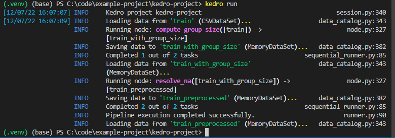
Looks like our pipeline is working. And here is another important building block for a production pipeline: A good logger! Often your code will run on different platforms, in the cloud, on a server or a machine from a colleague. If there is a problem, a log can give you vital information what is going wrong and how to fix it. You can find a saved version of this log in logs/info.logs.
Combining pipelines
Feel free to carry on adding and converting your own pipelines for a bit of a challenge. Or download the completed project from my GitHub repository:
git clone --branch notebook2kedro https://github.com/picklejuicedev/kedro-tutorial.git
In total I created 4 pipelines:
data_proc: for pre-processing the training datadata_encode: for encoding the string based enumerationsdata_model: for creating the modeldata_report: for printing some performance metrics of the model
Each pipeline has a clear input and output. Now the nice thing about Kedro is that you don’t need to tell it which pipeline to run when. You connect them together by specifying inputs that are connected to outputs. For example the data_model pipeline takes the train_encoded dataset as input and returns a model, X_test and y_test. You can persist any dataset to storage by providing an entry for it in the catalog.yml file. So to keep the model, I added this entry to save it as pickle dataset:
model:
  type: pickle.PickleDataSet
  filepath: data/06_models/model.pickle
As before you can now run the complete pipeline with kedro run and you should see a finished model appear in the folder data/06_models.
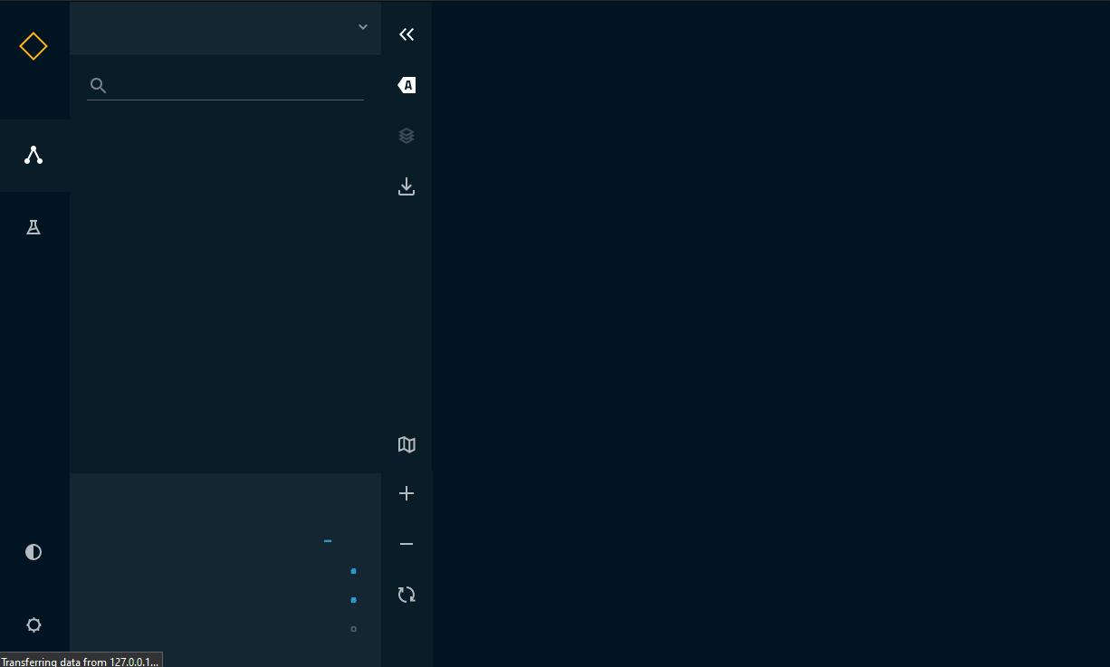
Visualising our pipelines
The last we will do in this tutorial is have a look at the pipeline we created using Kedro-Viz. First install it with:
pip install kedro-viz
Then use kedro viz to run it. You can now explore the different pipelines, datasets and nodes, even their implementation as code:
Conclusion
There you have it, one notebook converted into a Kedro pipeline that now provides the basis to take it to the next level. How about improving the model and creating an alternative path for some of the nodes? Or rewriting the reporting node to create some nice graphs instead of a simple console print out. Any of those changes can now be safely done because we have clearly defined processing blocks and interfaces between them. So as long as they take the same inputs and outputs you can easily create a new one.
Plus we can also consider some of the other software development best practices, such as automated testing to ensure the nodes and pipelines keep working the way we have designed them. We can also save this project to GitHub and share with colleagues. If we have kept the requirements.txt up to date, then they can run the same project and contribute. Or we can look at deploying our project to a cloud provider to rebuild our model automatically under certain conditions, maybe when new input data has arrived.
If you enjoyed this tutorial or have any suggestions for further Kedro tutorials, please leave a comment. Maybe some automated testing next?